Estimating a psychometric network with qgraph

We’re gonna need data

To estimate a psychological network we’re going to need data. Let’s take the 25 item Big-Five questionnaire from the psych package.

load_libraries <- function(){
  if (!require("dplyr"))
    install.packages("dplyr"); library(dplyr)
  if (!require("psych"))
    install.packages("psych"); library(psych)
  if(!require("qgraph"))
    install.packages("qgraph"); library(qgraph)
}

load_libraries()

df <- bfi[,1:25]
glimpse(df)

## Rows: 2,800
## Columns: 25
## $ A1 <int> 2, 2, 5, 4, 2, 6, 2, 4, 4, 2, 4, 2, 5, 5, 4, 4, 4, 5, 4, 4, 5, 1, 1~
## $ A2 <int> 4, 4, 4, 4, 3, 6, 5, 3, 3, 5, 4, 5, 5, 5, 5, 3, 6, 5, 4, 4, 4, 6, 5~
## $ A3 <int> 3, 5, 5, 6, 3, 5, 5, 1, 6, 6, 5, 5, 5, 5, 2, 6, 6, 5, 5, 6, 2, 6, 6~
## $ A4 <int> 4, 2, 4, 5, 4, 6, 3, 5, 3, 6, 6, 5, 6, 6, 2, 6, 2, 4, 4, 5, 1, 1, 5~
## $ A5 <int> 4, 5, 4, 5, 5, 5, 5, 1, 3, 5, 5, 5, 4, 6, 1, 3, 5, 5, 3, 5, 2, 5, 6~
## $ C1 <int> 2, 5, 4, 4, 4, 6, 5, 3, 6, 6, 4, 5, 5, 4, 5, 5, 4, 5, 5, 1, 4, 5, 4~
## $ C2 <int> 3, 4, 5, 4, 4, 6, 4, 2, 6, 5, 3, 4, 4, 4, 5, 5, 4, 5, 4, 1, 6, 4, 3~
## $ C3 <int> 3, 4, 4, 3, 5, 6, 4, 4, 3, 6, 5, 5, 3, 4, 5, 5, 4, 5, 5, 1, 5, 4, 2~
## $ C4 <int> 4, 3, 2, 5, 3, 1, 2, 2, 4, 2, 3, 4, 2, 2, 2, 3, 4, 4, 4, 5, 5, 2, 4~
## $ C5 <int> 4, 4, 5, 5, 2, 3, 3, 4, 5, 1, 2, 5, 2, 1, 2, 5, 4, 3, 6, 6, 4, 3, 5~
## $ E1 <int> 3, 1, 2, 5, 2, 2, 4, 3, 5, 2, 1, 3, 3, 2, 3, 1, 1, 2, 1, 1, 3, 1, 2~
## $ E2 <int> 3, 1, 4, 3, 2, 1, 3, 6, 3, 2, 3, 3, 3, 2, 4, 1, 2, 2, 2, 1, 3, 2, 1~
## $ E3 <int> 3, 6, 4, 4, 5, 6, 4, 4, NA, 4, 2, 4, 3, 4, 3, 6, 5, 4, 4, 4, 5, 4, ~
## $ E4 <int> 4, 4, 4, 4, 4, 5, 5, 2, 4, 5, 5, 5, 2, 6, 6, 6, 5, 6, 5, 5, 5, 3, 5~
## $ E5 <int> 4, 3, 5, 4, 5, 6, 5, 1, 3, 5, 4, 4, 4, 5, 5, 4, 5, 6, 5, 6, 4, 4, 2~
## $ N1 <int> 3, 3, 4, 2, 2, 3, 1, 6, 5, 5, 3, 4, 1, 1, 2, 4, 4, 6, 5, 5, 1, 2, 2~
## $ N2 <int> 4, 3, 5, 5, 3, 5, 2, 3, 5, 5, 3, 5, 2, 1, 4, 5, 4, 5, 6, 5, 3, 5, 2~
## $ N3 <int> 2, 3, 4, 2, 4, 2, 2, 2, 2, 5, 4, 3, 2, 1, 2, 4, 4, 5, 5, 5, 3, 5, 2~
## $ N4 <int> 2, 5, 2, 4, 4, 2, 1, 6, 3, 2, 2, 2, 2, 2, 2, 5, 4, 4, 5, 1, 2, 4, 2~
## $ N5 <int> 3, 5, 3, 1, 3, 3, 1, 4, 3, 4, 3, NA, 2, 1, 3, 5, 5, 4, 2, 1, 1, 6, ~
## $ O1 <int> 3, 4, 4, 3, 3, 4, 5, 3, 6, 5, 5, 4, 4, 5, 5, 6, 5, 5, 4, 4, 6, 5, 6~
## $ O2 <int> 6, 2, 2, 3, 3, 3, 2, 2, 6, 1, 3, 6, 2, 3, 2, 6, 1, 1, 2, 1, 1, 1, 1~
## $ O3 <int> 3, 4, 5, 4, 4, 5, 5, 4, 6, 5, 5, 4, 4, 4, 5, 6, 5, 4, 2, 5, 3, 6, 5~
## $ O4 <int> 4, 3, 5, 3, 3, 6, 6, 5, 6, 5, 6, 5, 5, 4, 5, 3, 6, 5, 4, 3, 2, 6, 5~
## $ O5 <int> 3, 3, 2, 5, 3, 1, 1, 3, 1, 2, 3, 4, 2, 4, 5, 2, 3, 4, 2, 2, 4, 2, 2~

Note that we have ordinal data. This is not problematic and we’ll mostyl deal with it using the cor_auto function from qgraph. The cor_auto function estimates a correlation matrix with the appropriate method for our data. This is done by automatically (hence the name) identifying our data type.

We have now three initial alternatives of estimation using the qgraph package:

1. Estimate network with a correlation matrix
2. Estimate network with a partial correlation matrix
3. Estimate network using EBICglasso

Before going into the actual code, let’s prepare this hyperparameter that’ll separe our nodes by groups.

traits <- rep(c('Agreeableness',
                'Conscientiousness',
                'Extraversion',
                'Neuroticism',
                'Openness'),
              each = 5)

1. Estimate network with a correlation matrix

network <- qgraph(cor_auto(df),
                  graph = 'cor',
                  layout = 'spring',
                  theme = 'colorblind',
                  groups = traits)

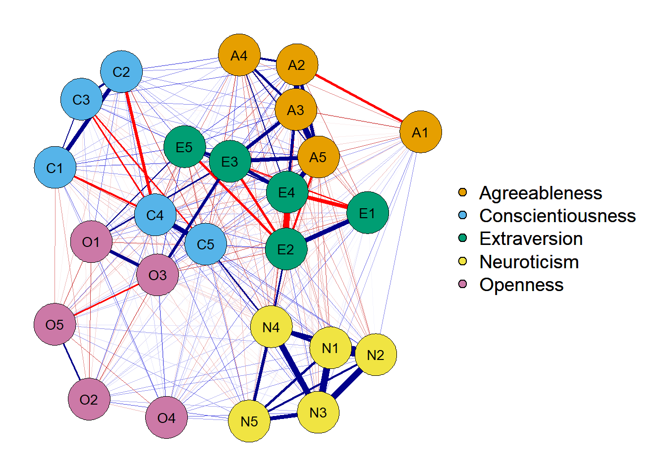
The correlation network plots the bivariate association between two variables. In this sense, when estimating an edge between two variables, it does not take into account the covariance existing between other variables. In my understanding, a graph like this would probably be used to show the bivariate association between a small number of variables.

2. Estimate network with a partial correlation matrix

network <- qgraph(cor_auto(df),
                  layout = 'spring',
                  graph = 'pcor', # note this new argument
                  theme = 'colorblind',
                  groups = traits)

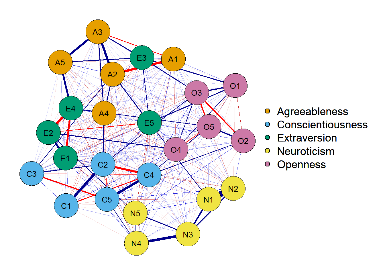
One way to take into account other variables' influence while estimating the unique association between two variables is by estimating a partial correlation matrix. This can be done with the graph = 'pcor' argument.

A graph that plots the unique association between two nodes is called a Gaussian Graphical Model (GGM). According to Burger et al. (in press), in a GGM the parameters are representing the unique association among two variables after conditioning on all other variables in the network.

3. Estimate network using EBICglasso

Note that the graph above is plotting the unique association between every two variables. A possible problem with the graph above is that we’re possibly plotting false positives since any partial correlation different than 0 is being shown. In that sense, a correlation of 0.02 would be plotted following the procedure above. The thing is: spurious correlations may not be present in the true model - they’re probably Type I errors.

We can prune and threshold our network to fix that, but for now I’d like to present another form of estimating a GGM while controling for Type I errors. This method is called EBICglasso - Extended Bayesian Information Criteria after estimating a graphical LASSO network (Foygel & Drton, 2010).

The code is fairly simple and, as you can see, the network is sparser (i.e., the network has less parameters, or edges). The only new argument should be the sample size used in estimating the variance-covariance matrix. This could be a number sampleSize = 2800 or you can directly pull this number from the dataframe (if you don’t have missing values), sampleSize = nrow(df).

network <- qgraph(cor_auto(df),
                  layout = 'spring',
                  graph = 'glasso',
                  sampleSize = nrow(df), # new argument!
                  theme = 'colorblind',
                  groups = traits)

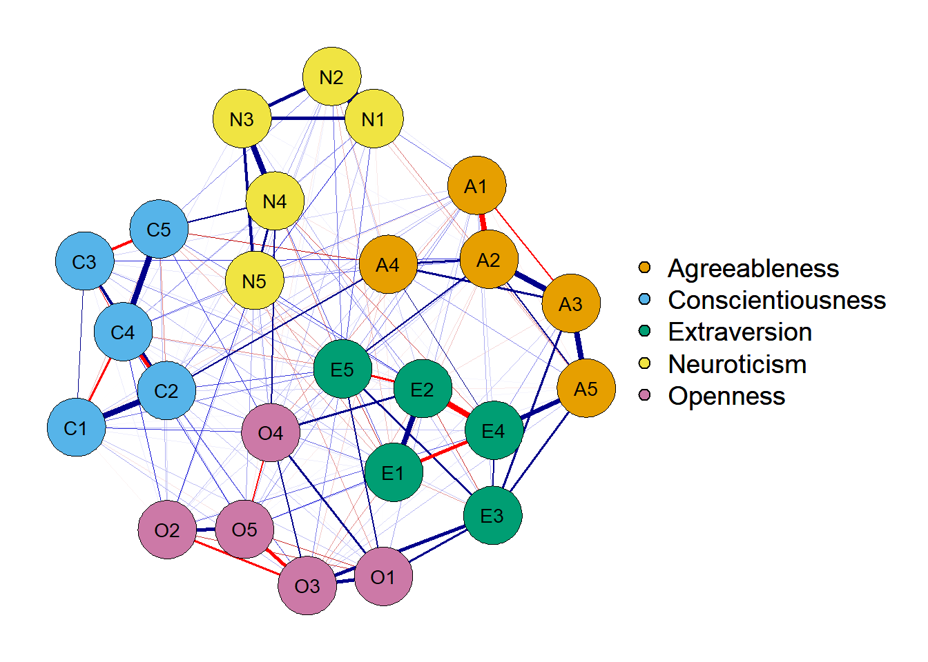Note that it’s sparser! How does it achieve that? The EBICglasso follows these steps:

1. Estimate partial correlation network S
2. Regularize S with the LASSO penalization n times using n different numbers of λ varying from 0 to 1.
3. Among the n networks, use the EBIC criterion to select the final network.

One important thing is that the EBIC uses a parameter called γ, that varies from 0 to 1. A value of γ = 0 aims toward discovery and allows for more Type I errors. A value of γ = 1 is conservative and will probably commit more Type II errors. The recommended value of γ is 0.5 according to Epskamp and Fried (2018). This is also the default in qgraph.

References

Burger, J., Isvoranu, A. M., Lunansky, G., Haslbeck, J. M. B., Epskamp, S., Hoekstra, R. H. A., Fried, E. I., Borsboom, D., & Blanken, T. F. (in press). Reporting standards for psychological network analyses in cross-sectional data. https://psyarxiv.com/4y9nz/

Costantini, G., Epskamp, S., Borsboom, D., Perugini, M., Mõttus, R., Waldorp, L. J., & Cramer, A. O. J. (2015). State of the aRt personality research: A tutorial on network analysis of personality data in R. Journal of Research in Personality, 54, 13–29. https://doi.org/10.1016/j.jrp.2014.07.003

Epskamp, S., Cramer, A. O. J, Waldorp, L. J., Schmittmann, V. D., Borsboom, D. (2012). qgraph: Network visualizations of relationships in psychometric data. Journal of Statistical Software, 48(4), 1–18. https://doi.org/10.18637/jss.v048.i04

Epskamp, S., & Fried, E. I. (2018). A tutorial on regularized partial correlation networks. Psychological Methods, 23(4), 617–634. https://doi.org/10.1037/met0000167

Foygel, R., & Drton, M. (2010). Extended Bayesian Information Criteria for gaussian graphical models. Proceedings of the 23rd International Conference on Neural Information Processing Systems, 604–612. arxiv.org/pdf/1011.6640.pdf