Exhausting all arguments on qgraph
Let's use it all!
By Gabriel R. R. in network psychometrics tutorials qgraph
August 21, 2021
TL;DR: I try to use all
qgraph::qgraph()’s arguments and fail miserably. Truth is, there’s just so many options, and most arguments didn’t apply to the data analysis I designed. Nevertheless, it was a great exercise and I learned A LOT more about qgraph.
Preparing the data
We’ll use all arguments on qgraph on this blog post. Well, we’ll either do that or die trying… Let’s again use the 25 item Big-Five questionnaire from the psych package. This time we’ll also load the items so we can create a pretty neat viz.
load_libraries <- function(){
  if (!require("dplyr"))
    install.packages("dplyr"); library(dplyr)
  if (!require("psych"))
    install.packages("psych"); library(psych)
  if(!require("qgraph"))
    install.packages("qgraph"); library(qgraph)
}

load_libraries()

# Data
df <- bfi[,1:25]

# Hyperparameters
# Group:
traits <- rep(c('Agreeableness',
                'Conscientiousness',
                'Extraversion',
                'Neuroticism',
                'Openness'),
              each = 5)

# Nodes:
items <- c(
  "Am indifferent to the feelings of others.",
  "Inquire about others' well-being.",
  "Know how to comfort others.",
  "Love children.",
  "Make people feel at ease.",
  "Am exacting in my work.",
  "Continue until everything is perfect.",
  "Do things according to a plan.",
  "Do things in a half-way manner.",
  "Waste my time.",
  "Don't talk a lot.",
  "Find it difficult to approach others.",
  "Know how to captivate people.",
  "Make friends easily.",
  "Take charge.",
  "Get angry easily.",
  "Get irritated easily.",
  "Have frequent mood swings.",
  "Often feel blue.",
  "Panic easily.",
  "Am full of ideas.",
  "Avoid difficult reading material.",
  "Carry the conversation to a higher level.",
  "Spend time reflecting on things.",
  "Will not probe deeply into a subject.")

# Neuroticism columns:
neuroticism <- c('N1', 'N2', 'N3', 'N4', 'N5')
Let’s create the biggest function ever created
Say we’re interested in Neuroticism. We want to look at its relationship with the other personality dimensions, its connections and its place in the network. In our function, we’ll make the neuroticism nodes bigger. And well… this is the only major change we’ll make. The rest of the arguments will remain practically the default ones. Oh!, another fancy thing we’ll do is plot the items and its dimensions in the graph.
network <-
  qgraph(
    input = cor_auto(df),

    #' *Important additional arguments* (p. 29)

    layout = 'spring', # 'circle', 'groups', 'circular'
    groups = traits, # list or vector
    minimum = 0, # min value to be plotted
    #' *maximum* =, max value to scale edge widths, default is absmax pcor(x,y)
    cut = 0, # value to initiate the scaling of edge widths
    details = F, # if T, min/max/cut is printed under the graph
    threshold = 0, # edges with abs value below this are REMOVED from estimation
    palette = 'colorblind', # 'rainbow', 'pastel', 'gray', 'R', 'ggplot2'
    theme = 'colorblind', # 'classic', 'gray', 'Hollywood', 'Borkulo', 'gimme',
    # 'TeamFortress', 'Reddit', 'Leuven', 'Fried'

    #' *Additional options for correlation/covariance matrices* (p. 30)

    graph = 'glasso', # 'cor', 'pcor'
    threshold = 'none', # remove edges based on significance testing; 'sig',
    # 'holm', 'hochberg', 'hommel', 'bonferroni', 'BH', 'BY', 'fdr', 'locfdr'
    sampleSize = nrow(df), # sample size, when graph="glasso" or minimum="sig"
    tuning = 0.5, # gamma argument
    lambda.min.ratio = 0.01, # min lambda value for glasso estimation
    gamma = 0.5, # just an alias for tuning, overwrites tuning
    refit = F, # should the optimal graph be refitted without LASSO?
    countDiagonal = F, # count diagonal in EBIC comp? generally F
    alpha = 0.05, # sig value for not showing edges if minimum = 'sig'
    bonf = F, # should a bonferroni correction be used if minimum = 'sig'?
    FDRcutoff = 0.9, # False-Discovery Rate cutoff if *threshold* = 'fdr'

    #' *Output arguments* (pp. 30-31)

    #mar = c(3, 3, 3, 3), # margins' vector c(bottom, left, top, rigth)
    #' *filetype* = 'R', can also be 'pdf', 'svg', 'tex', 'jpg', 'png', 'tiff'
    #' *filename* = 'graph', name of the file WITHOUT extension
    width = 7 * 1.4, # width of figure
    height = 7, # height of figure
    normalize = T, # graph's normalized to look the same for all sizes
    DoNotPlot = F, # useful to save plot without plotting
    plot = T, # should a new plot be made? if F, adds graph to existing plot
    rescale = T, # should layout be rescaled? best used with plot = F
    standAlone = F, # make output standalone LaTeX file if filetype = 'tex'

    #' *Graphical arguments*

    # Nodes (pp. 31-32)

    #color = rainbow(length(groups)), # vector with a color for each node
    vsize = ifelse(colnames(df) == neuroticism, 7.5, 6),
    # indicates node size, can be a vector with size for each node
    # default =  8*exp(-nNodes/80)+1
    #' *vsize2* = ..., node vertical size if shape = 'rectangle'
    node.width = 1, # scalar on value of vsize
    node.height = 1, # scalar on value of vsize2
    borders = T, # should borders be plotted?
    border.color = 'black', # color vector indicating colors of borders
    border.width = 0.5, # controls width of the border
    shape = 'circle', # 'square', 'triangle', 'diamond', 'ellipse', 'heart'
    #' *polygonList* = ..., list containing named lists for each element to
    #' include polygons
    vTrans = 255, # transparency of nodes, between 0 and 255 (no transparency)
    #' *subplots* = ..., list with as elements R expressions or NULL for
    #' each node. If an R expression, evaluated to create plot for the node.
    #' *subpars* = ..., list of graphical parameters to use in subplots
    #' *subplotbg* = ..., background to be used in subplots
    images = NA, # indicate file location of PNG of JPEG img to use as nodes
    noPar = F, # don't run the par function
    #' *pastel* = F, # should default colors be chosen from pastel colors?
    #' *rainbowStart* = ..., number from 0 to 1 indicating offset of rainbow
    usePCH = F, # nodes drawn using polygons or base R plotting symbols?
    node.resolution = 100, # resolution of nodes if usePCH = F
    # title = "Big-Five Inventory Psychometric Network", string graph title
    # title.cex = 0.5, size of title
    #' *preExpression* = ..., parsable string containing R code to be evaluated
    #' after opening a plot and before drawing the graph
    #' *postExpression* = ..., parsable string containing R code to be evaluated
    #' just before closing the device
    diag = F, # should diagonal also be plotted? Can also be 'col'

    # Node labels (pp. 32-33)

    #labels = T, # should labels be plotted?
    label.cex = 0.7, # scalar on label size
    label.color = 'black', # string on label colors
    label.prop = 0.9, # proportion of the width of the node that the label scales
    label.norm = "OOO", # normalize width of label size in nodes
    label.scale = T, # should labels be scaled to fit the node?
    label.scale.equal = T, # should labels have same font size?
    #' *label.font* = ..., # integer specifying the label font of nodes
    #' *label.fill.vertical* = ..., scalar indicating max prop to fill a node
    #' *label.fill.horizontal* = ..., scalar indicating max prop to fill a node
    node.label.offset = c(0.5,0.5), # where should label be centered, (x, y)
    node.label.position = NULL, # set specific positions of node labels

    # Edges (pp. 33-34)
    #' *esize* = ..., size of largest edge
    #' *edge.width* = ..., size of largest edge
    #' *edge.color* = ..., size of largest edge
    # posCol = c("#009900", "darkgreen"), color of positive edges
    negCol = c("#BF0000","red"), # color of negative edges
    unCol = "#808080", # default edge color of unweighted graphs
    probCol = "blue", # color of probability nodes
    negDashed = T, # should negative edges be dashed?
    probabilityEdges = F, # do edges indicate probabilities?
    colFactor = 1, # exponentially transforms color int. of relative strength 1
    trans = T, # should edges fade to white?
    fade = T, # should edges fade?
    loopRotation = NA, # vector for each node assigning rotation in radians
    loop = 1, # if diag = T, scales the size of the loop
    lty = 1, # line type, see 'par'
    #' *edgeConnectPoints* = ..., specifies the point for each edge to which it
    #' connects to a node, in radians

    # Edge curvature (pp. 34-35)
    # curve = NA, # single value, a vector list, weight matrix or NA (default)
    curveAll = T, # logical indicating if all edges should be curved
    curveDefault = 0.5, # default is 1
    curveShape = -1, # shape of the curve, as used in xspline
    curveScale = T, # should curve scale with distance between nodes?
    curveScaleNodeCorrection = T, # discable node correction in curveScale
    curvePivot = F, # can be logical or numeric, this can be used to make
    # straight edges as curves with knicks in them.
    curvePivotShape = 0.25, # shape of edge pivot, default is 0.25
    parallelEdge = F, # draw parallel straight edges rather than curved ones?
    parallelAngle = NA, # distance in radians an edge is shifted
    parallelAngleDefault = pi/6, # angle of the edge furthest from the center

    # Edge labels (p. 35)
    edge.labels = F, # if T, numeric is plotted. if F, nothing is.
    edge.label.cex = 1, # single number or number per edge
    edge.label.bg = T, # plot a white background behind number
    edge.label.margin = 0, # margin of the background bow around the edge label
    edge.label.position = 0.5, # vector between 0 and 1, 0.5 is middle
    #' *edge.label.font* = ..., numeric specifying the label font of edges
    #' *edge.label.color* = ..., character vector indicating color of edge label

    # Layout (p. 35)
    repulsion = 1, # setting to lower values will cause nodes to repulse each
    # other less. This is useful if few unconnected nodes cause the giant
    # component to visually be clustered too much in the same place.
    #' *layout.par* = ..., list of arguments passed to
    #' qgraph.layout.fruchtermanreingold()
    layoutRound = T, # should weights be rounded before computing layouts?
    #' *layout.control* = ..., scalar on the size of the circles created
    aspect = F, # should the original aspect ratio be maintained if rescaled?
    rotation = 0, # rotate the circles created with the circular layout;
    # contains the rotation in radian for each group of nodes

    # Legend (p. 35-36)
    legend = T, # should a legend be plotted?
    legend.cex = 0.27, # scalar of the legend
    legend.mode = 'style2', # default is 'style1', different way to show legend
    GLratio = 2.5, # relative size of graph compared to the layout
    layoutScale = c(1, 1), # vector with a scalar for respectively the x and y
    # coordinates of the layout. Setting this to c(2, 2) makes plot twice as
    # big. This can be used with layoutOffset to determine the graph's placement.
    layoutOffset = c(0,0), # vector with the offset to the x and coordinates of
    # the center of the graph
    nodeNames = items, # names for each node to plot in legend

    # Background (p. 36)
    bg = F, # should node colors cast a light in the background?
    # can also be a color...
    bgcontrol = 6, # the higher, the less light each node gives if bg = T
    bgres = 100, # (default) square root of the number of pixels used in bg = T

    # Generical graphical arguments (p. 36)
    #' *pty* = ..., see 'par'
    gray = F, # should the graph be plotted in grayscale colors?
    font = 2, # integer specifying default font for node and edge labels

    # Arguments for directed graphs (p. 36)
    directed = F, # are edges directed? can be logical vector/matrix
    arrows = F, # should arrows be plotted? can be a number
    arrowAngle = pi/8, # (default for unweighted) and pi/4 for weighted
    #' *azise* = ..., size of the arrowhead
    open = F, # should arrowheads be open?
    bidirectional = F, # should directional edges between nodes have two edges?

    # Arguments for graphs based on significance values (p. 37)
    mode = "strength", # defines mode used for coloring edges, can be "sig" too
    alpha = 0.05, # if minimum = "sig" , sig level for not showing edges
    #' *sigScale* = ..., fybctuib ysed ti scake tge edges if mode = "sig"
    bonf = F, # should bonferronni correction be applied?

    # Arguments for plotting scores on nodes (p. 37)
    #' *scores* = ..., vector used to plot scores of an individual on the test
    #' *scores.range* = ..., vector of length two indicating the range of scores

    # Arguments for manually defining graphs (p. 37)
    #' *mode* = ..., mode can also be used to make the weights matrix correspond
    #' directly with the width of the edges
    edge.color = NA, # argument used to overwrite the colors, can be a single
    # value or vector/matrix with a color for each edge

    # Arguments for knots (tying together edges) (p. 37)
    #' *knots* = ..., argument used to tie edges together in their center,
    #' useful for indicating interaction effects. Can be a list where each
    #' element is a vector containing the edge numbers that should be knotted.
    #' *knot.size* = 1, size of the knots
    #' *knot.color* = NA, color of the knots
    #' *knot.borders* = F, should a border be plotted around the knot?
    #' *knot.border.color* = 'black', color of the know borders
    #' *knot.border.width* = 1, width of the knot borders

    # Arguments for bars (p. 38)
    #' *means* = ..., vector with means for every node or NA, will plot a
    #' vertical bar at the location of the mean between meanRange values
    #' *SDs* = ..., vector with SDs for every node or NA, will plot an error bar
    #' of 2 times this value around the means location
    #' *meanRange* = ..., range of the means argument
    #' *bars* = ..., a list with for each node or vector with values between 0-1
    #' indicating where bars should be placed inside the node
    #' *barSide* = ..., integer for each node indicating at which side the bars
    #' should be drawn. 1, 2, 3 or 4: bottom, left, top or right respectively.
    #' *barColor* = ..., vector with for each node indicating color of bars
    #' *barLength* = 0.5, vector indicating relative length of bars for each
    #' node compared to the node size
    #' *barsAtSide* = F, should bars be drawn at the side of a node?

    # Arguments for pies (p. 38)
    #' *pie* = ..., vector with values between 0-1 for each node or just one
    #' value for all nodes. This will make the border of nodes a pie chart.
    #' *pieBorder* = 0.15, size of the pie chart in the border, between 0-1
    #' *pieColor* = ..., colors of the pie plot parts, can be a vector with a
    #' value for each node or list with multiple values if there are more parts
    #' *pieColor2* = 'white', final color of the pie chart
    #' *pieStart* = ..., vector with values between 0-1 for each node or just
    #' one value for all nodes indicating the starting point of the pie chart.
    #' *pieDarken* = ..., vector with values between 0-1 for each node or just
    #' one value for all nodes indicating how much darker the pie border is
    #' *piePastel* = F, pastel colors to fill pie chart parts when >= 2 blocks?
    #' *pieCImid* = ..., vector with values between 0-1 for each node or just
    #' one value for all nodes indicating center point of confidence region
    #' *pieCIlower* = ..., vector with values between 0-1 for each node or just
    #' one value for all nodes indicating lower point of confidence region
    #' *pieCIupper* = ..., vector with values between 0-1 for each node or just
    #' one value for all nodes indicating upper point of confidence region
    #' *pieCIpointcex* = 0.01, vector with values between 0-1 for each node or
    #' just one value for all nodes indicating size of the point estimate
    #' *pieCIpointcex* = 'black', vector with values between 0-1 for each node
    #' or just one value for all nodes indicating color of the point estimate

    # Additional arguments (p. 39)
    edgelist = F, # is input an edgelist?
    weighted = T, # is input weighted?
    nNodes = 25 # number of nodes, only specified if edgelist = T
    # XKCD = T, if T, graph is plotted in XKCD style based on
    #' http://stackoverflow.com/a/12680841/567015
  )
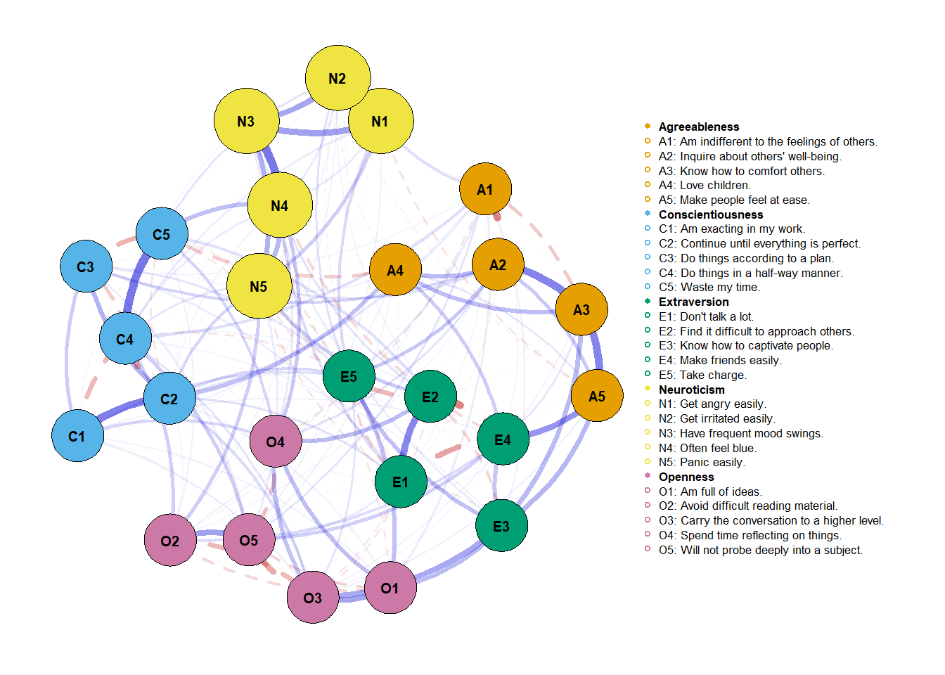 There we go! A personalyzed network graph.
Making the same graph with a smaller function
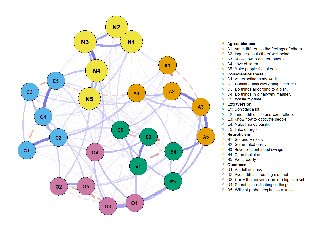
If you read the function, you probably noticed that a lot of values used on the arguments were default. To facilitate my future work, I’ll now create the same graph without the spare arguments from before.
network <-
  qgraph(
    input = cor_auto(df),

    #' *Important additional arguments* (p. 29)

    layout = 'spring', # 'circle', 'groups', 'circular'
    groups = traits, # list or vector
    minimum = 0, # min value to be plotted
    #' *maximum* =, max value to scale edge widths, default is absmax pcor(x,y)
    cut = 0, # value to initiate the scaling of edge widths
    palette = 'colorblind', # 'rainbow', 'pastel', 'gray', 'R', 'ggplot2'
    theme = 'colorblind', # 'classic', 'gray', 'Hollywood', 'Borkulo', 'gimme',
    # 'TeamFortress', 'Reddit', 'Leuven', 'Fried'

    #' *Additional options for correlation/covariance matrices* (p. 30)

    graph = 'glasso', # 'cor', 'pcor'
    sampleSize = nrow(df), # sample size, when graph="glasso" or minimum="sig"

    #' *Output arguments* (pp. 30-31)
    width = 7 * 1.4, # width of figure
    height = 7, # height of figure

    #' *Graphical arguments*

    # Nodes (pp. 31-32)

    vsize = ifelse(colnames(df) == neuroticism, 7.5, 6),
    # indicates node size, can be a vector with size for each node
    # default =  8*exp(-nNodes/80)+1
    border.width = 0.5, # controls width of the border

    # Node labels (pp. 32-33)
    label.cex = 0.7, # scalar on label size
    label.color = 'black', # string on label colors
    label.prop = 0.9, # proportion of the width of the node that the label scales

    # Edges (pp. 33-34)
    negDashed = T, # should negative edges be dashed?

    # Edge curvature (pp. 34-35)
    # curve = NA, # single value, a vector list, weight matrix or NA (default)
    curveAll = T, # logical indicating if all edges should be curved
    curveDefault = 0.5, # default is 1

    # Legend (p. 35-36)
    legend.cex = 0.27, # scalar of the legend
    legend.mode = 'style2', # default is 'style1', different way to show legend
    nodeNames = items, # names for each node to plot in legend

    # Generical graphical arguments (p. 36)
    font = 2 # integer specifying default font for node and edge labels
  )
Estimate network with a “cool” background
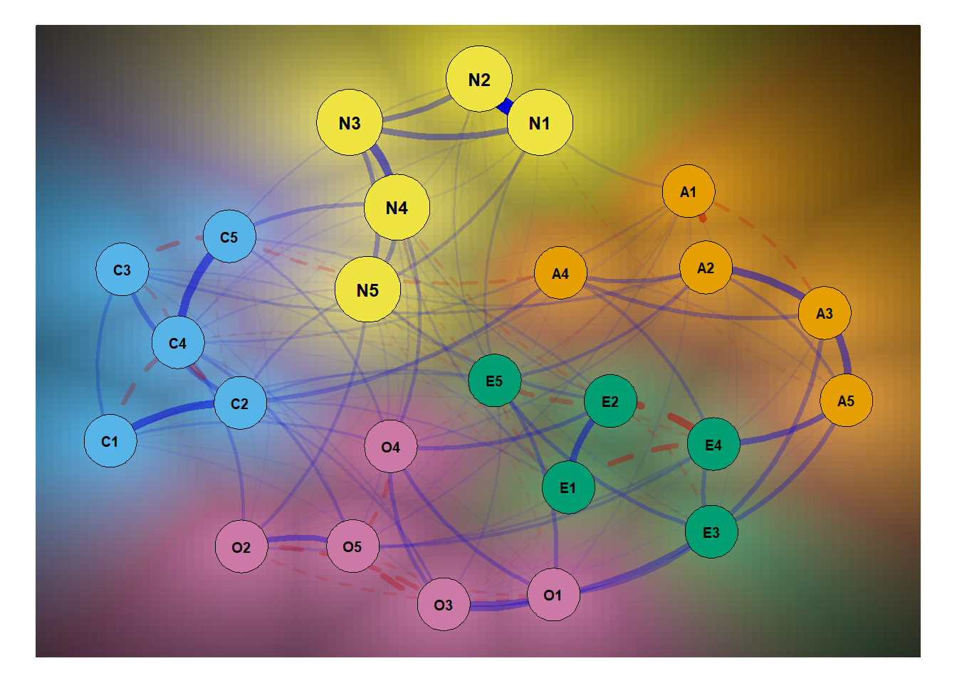
One cool thing I found out during this is the bg = T argument.
Basically, this argument lets the light shine through the node
and onto the background. It’s quite interesting. It’s probably
more useful if we have a bunch of nodes and various groupings.
But, for now, let’s see what we can get with this…
network <-
  qgraph(
    input = cor_auto(df),

    #' *Important additional arguments* (p. 29)

    layout = 'spring', # 'circle', 'groups', 'circular'
    groups = traits, # list or vector
    minimum = 0, # min value to be plotted
    #' *maximum* =, max value to scale edge widths, default is absmax pcor(x,y)
    cut = 0, # value to initiate the scaling of edge widths
    palette = 'colorblind', # 'rainbow', 'pastel', 'gray', 'R', 'ggplot2'
    theme = 'colorblind', # 'classic', 'gray', 'Hollywood', 'Borkulo', 'gimme',
    # 'TeamFortress', 'Reddit', 'Leuven', 'Fried'

    #' *Additional options for correlation/covariance matrices* (p. 30)

    graph = 'glasso', # 'cor', 'pcor'
    sampleSize = nrow(df), # sample size, when graph="glasso" or minimum="sig"

    #' *Output arguments* (pp. 30-31)
    width = 7 * 1.4, # width of figure
    height = 7, # height of figure

    #' *Graphical arguments*

    # Nodes (pp. 31-32)

    vsize = ifelse(colnames(df) == neuroticism, 7.5, 6),
    # indicates node size, can be a vector with size for each node
    # default =  8*exp(-nNodes/80)+1
    border.width = 0.5, # controls width of the border

    # Node labels (pp. 32-33)
    label.cex = 0.7, # scalar on label size
    label.color = 'black', # string on label colors
    label.prop = 0.9, # proportion of the width of the node that the label scales

    # Edges (pp. 33-34)
    negDashed = T, # should negative edges be dashed?

    # Edge curvature (pp. 34-35)
    # curve = NA, # single value, a vector list, weight matrix or NA (default)
    curveAll = T, # logical indicating if all edges should be curved
    curveDefault = 0.5, # default is 1

    # Legend (p. 35-36)
    legend = F,

    # Generical graphical arguments (p. 36)
    font = 2, # integer specifying default font for node and edge labels

    # Background (p. 36)
    bg = T, # should node colors cast a light in the background?
    # can also be a color...
    bgcontrol = 3 # the higher, the less light each node gives, default is 6
  )
 That’s it for now!
References
Costantini, G., Epskamp, S., Borsboom, D., Perugini, M., Mõttus, R., Waldorp, L. J., & Cramer, A. O. J. (2015). State of the aRt personality research: A tutorial on network analysis of personality data in R. Journal of Research in Personality, 54, 13–29. https://doi.org/10.1016/j.jrp.2014.07.003
Epskamp, S., Cramer, A. O. J, Waldorp, L. J., Schmittmann, V. D., Borsboom, D. (2012). qgraph: Network visualizations of relationships in psychometric data. Journal of Statistical Software, 48(4), 1–18. https://doi.org/10.18637/jss.v048.i04
- Posted on:
- August 21, 2021
- Length:
- 17 minute read, 3523 words
- Categories:
- network psychometrics tutorials qgraph
- See Also: