bootnet: A tutorial on estimating accuracy and stability
By Gabriel R. R. in tutorials bootnet network psychometrics
September 27, 2021
BFI dataset
We’ll use the Big-Five Inventory dataset to estimate accuracy and stability measures using the bootnet package. After cleaning our data and stablishing the groupings of variables, we’ll look at:
- Estimation with bootnet
- Stability of edge weights
- Stability of centrality measures
- Stability of differences in edge weights or in centrality measures
- Reporting our findings
load_libraries <- function(){
  if (!require("bootnet"))
    install.packages("bootnet"); library(bootnet) # select() and mutate()
  if (!require("dplyr"))
    install.packages("dplyr"); library(dplyr) # select() and mutate()
  if (!require("magrittr"))
    install.packages("magrittr"); library(magrittr) # %<>% operator
  if (!require("psych"))
    install.packages("psych"); library(psych)
  if (!require("qgraph"))
    install.packages("qgraph"); library(qgraph)
}

load_libraries()

# Data:
df <- bfi[,1:25]

# Group:
traits <- rep(c('Agreeableness',
                'Conscientiousness',
                'Extraversion',
                'Neuroticism',
                'Openness'),
              each = 5)

# Nodes:
items <- c(
  "Am indifferent to the feelings of others.",
  "Inquire about others' well-being.",
  "Know how to comfort others.",
  "Love children.",
  "Make people feel at ease.",
  "Am exacting in my work.",
  "Continue until everything is perfect.",
  "Do things according to a plan.",
  "Do things in a half-way manner.",
  "Waste my time.",
  "Don't talk a lot.",
  "Find it difficult to approach others.",
  "Know how to captivate people.",
  "Make friends easily.",
  "Take charge.",
  "Get angry easily.",
  "Get irritated easily.",
  "Have frequent mood swings.",
  "Often feel blue.",
  "Panic easily.",
  "Am full of ideas.",
  "Avoid difficult reading material.",
  "Carry the conversation to a higher level.",
  "Spend time reflecting on things.",
  "Will not probe deeply into a subject.")
Estimation with bootnet
Estimation with bootnet is very simple. We only have to use the function
estimateNetwork() in our data object.
Note that in the bootnet documentation, there are other functions specified in
estimateNetwork(). The network estimation occurs in these ghost functions that
we can change directly in estimateNetwork() via the default = parameter.
Say we want to estimate an EBIGglasso network. To do that, we simply give the
function the data object and the specification default = "EBICglasso". This’ll
open the ghost function bootnet_EBICglasso, and we can now access its
parameters and make our changes. Say we’re working with binary data (0s and 1s)
and we want to estimate and Ising model, we specify default = "IsingFit".
This’ll open the ghost function bootnet_IsingFit that’s now available for
modification.
Let’s create an object with our estimated network.
Note that the option
default = "EBICglasso"specifies gamma to be 0.5 in the tuning parameter.
network <- estimateNetwork(df,
                           default = "EBICglasso",
                           corMethod = "spearman")

class(network)
## [1] "bootnetResult" "list"
What we have now is called a bootnetResult. This is what we’ll use to
estimate stability and network accuracy. To plot our network, we can use the
plot() function in R, giving the same parameters found in the qgraph package.
plot(network,
     layout = "spring",
     groups = traits,
     label.cex = 0.7, # scalar on label size
     label.color = 'black', # string on label colors
     label.prop = 0.9, # proportion of the width of the node that the label scales

     # Edges (pp. 33-34)
     negDashed = T, # should negative edges be dashed?

     # Legend (p. 35-36)
     legend.cex = 0.27, # scalar of the legend
     legend.mode = 'style2', # default is 'style1'
     nodeNames = items, # names for each node to plot in legend

     # Generical graphical arguments (p. 36)
     font = 2)
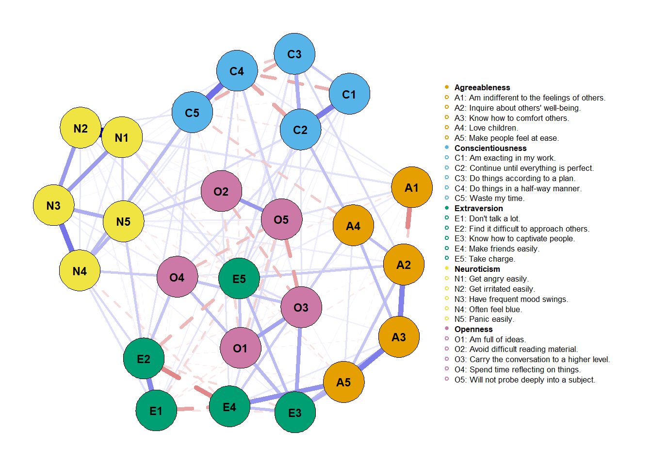
Another thing we can do is simply run the object and get a small summary of our estimated network.
network
##
## === Estimated network ===
## Number of nodes: 25
## Number of non-zero edges: 168 / 300
## Mean weight: 0.01947714
## Network stored in x$graph
##
## Default set used: EBICglasso
##
## Use plot(x) to plot estimated network
## Use bootnet(x) to bootstrap edge weights and centrality indices
##
## Relevant references:
##
##  	Friedman, J. H., Hastie, T., & Tibshirani, R. (2008). Sparse inverse covariance estimation with the graphical lasso. Biostatistics, 9 (3), 432-441.
## 	Foygel, R., & Drton, M. (2010). Extended Bayesian information criteria for Gaussian graphical models.
## 	Friedman, J. H., Hastie, T., & Tibshirani, R. (2014). glasso: Graphical lasso estimation of gaussian graphical models. Retrieved from https://CRAN.R-project.org/package=glasso
## 	Epskamp, S., Cramer, A., Waldorp, L., Schmittmann, V. D., & Borsboom, D. (2012). qgraph: Network visualizations of relationships in psychometric data. Journal of Statistical Software, 48 (1), 1-18.
## 	Epskamp, S., Borsboom, D., & Fried, E. I. (2016). Estimating psychological networks and their accuracy: a tutorial paper. arXiv preprint, arXiv:1604.08462.
We seem to have a highly dense network since 168/300 connections were made - which is equal to 56% of all possible connections.
Stability of edge weights
We’re going to use our bootnetResult object to estimate the stability of edge weights. From now on, our estimates will come from bootstrap samples. For our initial procedures, we’ll use nonparametric bootstraps (sampling cases randomly with replacement).
What will happen is:
- We’ll create a bootstrapped sample.
- We’ll now replicate the same estimation we used with our sample.
- Store this bootstrapped sample edge weights.
- Repeat steps 1 to 3 n times.
We’ll then be able to estimate how much our edge weights for each connection varied with a 95% confidence interval (i.e., without the top 2.5% and the bottom 2.5% edge weights for that connection).
Note: the procedure below can take a while. I established
nCores = 8to use all my computer power to calculate the bootstrapped samples and its estimates.
bootnet_nonpar <- bootnet(network,
                          nBoots = 1000, # number of boot samples
                          nCores = 8)

# Looking at the width of variation
plot(bootnet_nonpar,
     labels = FALSE,
     order = "sample")
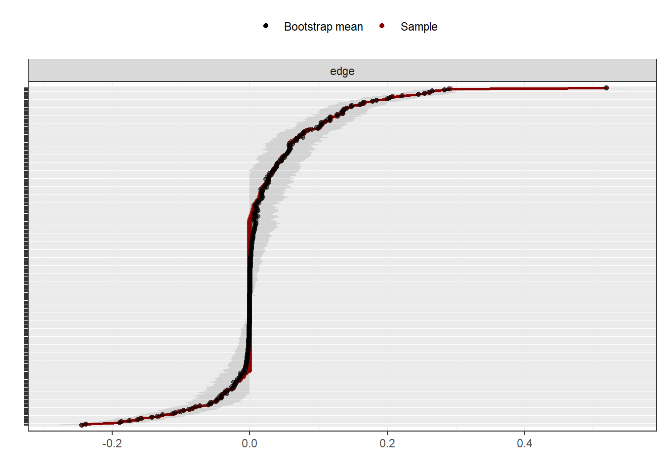
The graph above shows the edge estimate in the sample (), the mean edge estimate in the bootstrapped samples and the 95% confidence interval band from the bootstraps edge weights. Visually, we can notice how some edge weights are more accurate than others (have a lower band). At the same time, we notice how the majority of edges closer to 0 seem to be non-significant (i.e., they cross 0 in the bootstrapped samples).
Stability of centrality measures
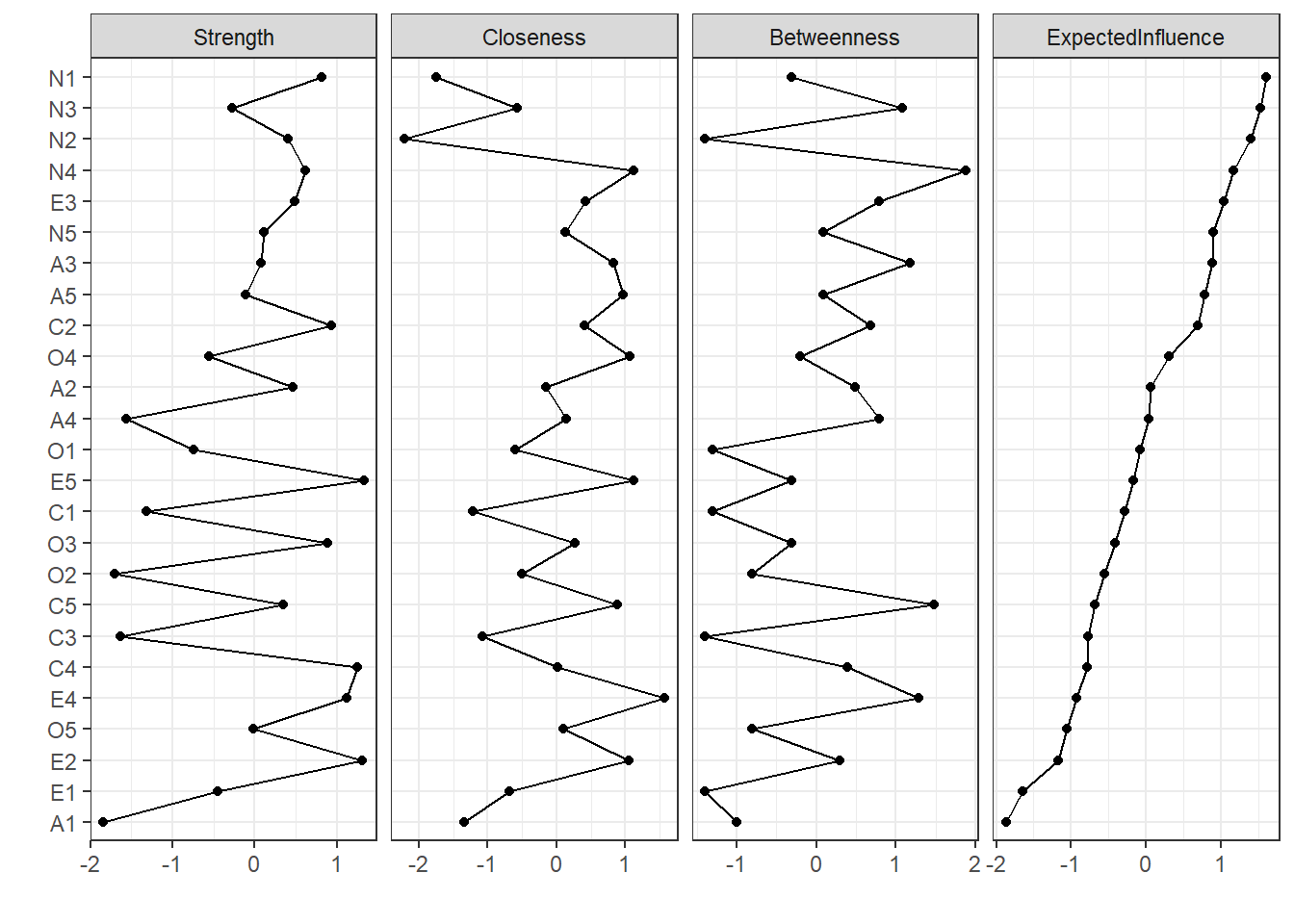
We’re going to use our bootnetResult object to estimate the stability of centrality measures. First, let’s take a look at our centrality measures:
centralityPlot(network, include = "all", orderBy = "ExpectedInfluence")
 The question we’re making in this section is the following: are our centrality
indices realiable? How much do they change as we change our sample?
Specifically, we’ll test if centrality indices reflect the relationship between
nodes or if these values are influenced by subsets of our sample.
The question we’re making in this section is the following: are our centrality
indices realiable? How much do they change as we change our sample?
Specifically, we’ll test if centrality indices reflect the relationship between
nodes or if these values are influenced by subsets of our sample.
To do that, we’ll create more bootstrapped samples. This time, we’ll do that with a case-dropping bootstrap. This occurs when we randomly exclude cases from our original dataset, creating a new dataset. What this does is:
What will happen is:
- We’ll create n bootstrapped samples by randomly excluding X% of our sample.
- After creating these n case dropped bootstraps for X%, we then calculate the networks and centrality indices for each of these n networks.
- We store our statistics and then proceed to excluding a bigger percentage from our sample.
- Repeat steps 1 to 3 until we go from excluding 10% of our sample to 70%.
bootnet_case_dropping <- bootnet(network,
nBoots = 2500,
type = "case",
nCores = 8,
statistics = c('strength',
'expectedInfluence',
'betweenness',
'closeness'))
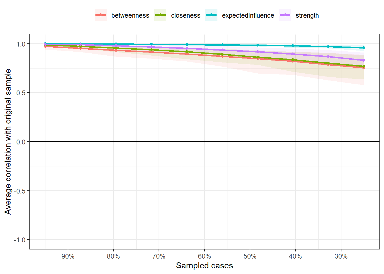
plot(bootnet_case_dropping, 'all')
Note we’re already specifying which centrality measures we want to store. As
such, if we’re interested in only one specific centrality indice
(say, strength), we can shorten our computation time by specifying
statistics = "strength".
What is this plot? The plot is indicating the mean correlation between each of the four centrality indices (differentiated by colors) in our sample compared to our 1000 bootstrapped samples for each exclusion interval. Note that r > 0.9 when we dropped only 10% of our sample. This indicates that these centrality indices are practically the same and stable for this interval. What we’re interested in is what happens in 30%. If r < 0.5 in the 30% sampled cases, there seems to be only a weak to moderate correlation between our original sample’s centrality indices and our bootstrapped samples' values.
To avoid having to check that by eyesight, Epskamp et al. (2018) developed a
statistic called Correlation-Stability Coefficient (CS-Coefficient). This
indicates the mean percentage of our sample that can be dropped to preserve a
correlation of r = 0.7 between our sample’s centrality indices and our
case-dropped bootstraps' centrality indices. Note: r = 0.7 can be changed. The
idea is: if we can drop a lot of cases from our original sample and still
preserve a high correlation between centrality indices, we have a pretty solid
notion that these nodes are not being influenced by sample characteristics
(i.e., they’re probably stable in our population). We can investigate
CS-Coefficiente(r = 0.7) using the corStability() function from bootnet.
As an input, we provide the object with our case-dropping bootstrap.
corStability(bootnet_case_dropping)
## === Correlation Stability Analysis ===
##
## Sampling levels tested:
##    nPerson Drop%   n
## 1      700  75.0 254
## 2      918  67.2 244
## 3     1136  59.4 217
## 4     1353  51.7 230
## 5     1571  43.9 261
## 6     1789  36.1 259
## 7     2007  28.3 259
## 8     2224  20.6 273
## 9     2442  12.8 245
## 10    2660   5.0 258
##
## Maximum drop proportions to retain correlation of 0.7 in at least 95% of the samples:
##
## betweenness: 0.594
##   - For more accuracy, run bootnet(..., caseMin = 0.517, caseMax = 0.672)
##
## closeness: 0.594
##   - For more accuracy, run bootnet(..., caseMin = 0.517, caseMax = 0.672)
##
## expectedInfluence: 0.75 (CS-coefficient is highest level tested)
##   - For more accuracy, run bootnet(..., caseMin = 0.672, caseMax = 1)
##
## strength: 0.75 (CS-coefficient is highest level tested)
##   - For more accuracy, run bootnet(..., caseMin = 0.672, caseMax = 1)
##
## Accuracy can also be increased by increasing both 'nBoots' and 'caseN'.
Note that all CS-Coefficients are above 0.5. Epskamp et al. (2018) suggest that “the CS-coefficient should not be below 0.25, and preferably above 0.5.” This tells us we can make solid interpretations based on our centrality indices, especially for strength (CS(cor = 0.7) = 0.75) and expected influence (CS(cor = 0.7) = 0.75).
Stability of differences in edge weights or in centrality measures
We’re going to use our bootnetResult object to estimate the stability of possible differences in edge weights and/or in centrality measures.
This is a pretty simple test. What we’re asking is: the edge weight and/or centrality indices difference we encountered in our sample occurs evenly throughout our bootstrapped samples? This is tested checking our sample’s difference and comparing it to a 95% interval of all bootstraps statistics for that specific difference.
Above, we saw that nodes N1 and N4 shows the highest strength values for neuroticism, in that order. Let’s ask: is this a noticeable difference? Can we interpret that N1 has stronger connections than N4 or is this difference unstable throughout or bootstrap samples?
To do this, we’ll again use our non-parametric bootstrap results.
differenceTest(bootnet_nonpar,
               "N1", "N4",
               measure = "strength")
##   id1 id2  measure      lower      upper significant
## 1  N1  N4 strength -0.1404831 0.09632485       FALSE
As we can see, there isn’t a significant difference between the two nodes'
strength. How can we talk about significance? Well, this test was called
bootstrap significance testing, in the sense that if we go from the lower to
the upper statistics crossing 0, there doesn’t seem to be a significant
difference between the two nodes in the population. The lower and upper interval
correspond to the 2.5 percentile difference and 97.5 percentile difference,
establishing a 95% confidence interval. The 95% interval can be changed with the
alpha argument in differenceTest(..., alpha = 0.05). If we want, we can have
a 90% confidence interval writing differenceTest(..., alpha = 0.10).
Now, let’s check if two edge weights have stable differences. We’ll look at N1 and N2, and N1 and N5. We can do that in two ways, which will be presented below:
differenceTest(bootnet_nonpar,
               "N1--N2",
               "N1--N5",
               measure = "edge")
##      id1    id2 measure      lower      upper significant
## 1 N1--N2 N1--N5    edge -0.4668853 -0.3634959        TRUE
There seems to be a significant difference between the two edges!
To get the same results, we could also run:
differenceTest(bootnet_nonpar,
               x = "N1", x2 = "N2", # N1--N2
               y = "N1", y2 = "N5", # N1--N5
               measure = "edge")
Reporting our findings
If we’re writing an article using what we’ve learned here, we’d have to report what we’ve done in our “Data Analysis” topic in the Methods section and also report our results in the Results section. I’ll write below how I’d do it, based on Burger et al. (in press) recommendations.
Data Analysis
Analysis were conducted in R (version 4.1.1) in September 27th of 2021. A partial correlation network was estimated using a Spearman correlation matrix, using LASSO regularization (Least Absolute Shrinkage and Selection Operator; Friedman et al., 2008). After LASSO regularization, a network was selected using Extended Bayesian Information Criterion (EBIC; Foygel & Drton, 2010), with γ = 0.5. This estimation procedure were condcuted using the qgraph package (Epskamp et al., 2012; versão 1.6.9). Network visualization was possible using qgraph; network colors were fixed to be colorblind friendly (blue meaning positive and red meaning negative edge weights) and negative edges were dashed.
Looking to estimate edge and centrality stability, bootnet package was used (Epskamp et al., 2018; versão 1.4.3). Non-parametric bootstrap (resampling rows with replacement) was used to create 1000 samples to estimate edge weights stability. Case-dropping subset bootstrap samples (n = 1000) were used to estimate the stability of centrality indices. Correlation Stability coefficient for correlation values equal or above to r = 0.7 (CS-coefficient(r = 0.7); Epskamp et al., 2018) were used to measure stability of centrality indices. CS-coefficient indicates the percentage of our sample that can be dropped to mantain, with a 95% confidence interval, correlation values equal or above to r = 0.7 between our sample’s centrality indices and our bootstrapped samples' centrality indices.
Results
Graph on the relations between personality items can be visualized in Figure 1. The network was made up of 25 nodes, mean edge weight was 0.019 and network density was somewhat high: 168 out of 300 possible connections were observed, consisting of 56% of all possible connections.
Stabilty of edge weights (Figure 2) shows stable connections and all centrality measures present CS(cor = 0.7) > 0.59. Overall, we can conclude that our results can be generalized to the population. On that note, centrality measures are presented on Figure 3, ordered by expected influence.
[More notes on specific nodes and connections. Highlight strong and influent nodes. Hypothesize about specific edges and so on…]
References
Burger, J., Isvoranu, A. M., Lunansky, G., Haslbeck, J. M. B., Epskamp, S., Hoekstra, R. H. A., Fried, E. I., Borsboom, D., & Blanken, T. F. (in press). Reporting standards for psychological network analyses in cross-sectional data. https://psyarxiv.com/4y9nz/
Epskamp, S., Cramer, A. O. J, Waldorp, L. J., Schmittmann, V. D., Borsboom, D. (2012). qgraph: Network visualizations of relationships in psychometric data. Journal of Statistical Software, 48(4), 1–18. https://doi.org/10.18637/jss.v048.i04
Epskamp, S., Borsboom, D., & Fried, E. I. (2017). Estimating psychological networks and their accuracy: A tutorial paper. Behavior Research Methods, 50(1), 195–212. https://doi.org/10.3758/s13428-017-0862-1
Foygel, R., & Drton, M. (2010). Extended Bayesian Information Criteria for gaussian graphical models. Proceedings of the 23rd International Conference on Neural Information Processing Systems, 604–612. https://arxiv.org/pdf/1011.6640.pdf
Friedman, J., Hastie, T., & Tibshirani, R. (2008). Sparse inverse covariance estimation with the graphical lasso. Biostatistics, 9(3), 432–441. https://doi.org/10.1093/biostatistics/kxm045
R Core Team. (2020). R: A language and environment for statistical computing (Version 4.1.1) [Computer software]. R Foundation for Statistical Computing. https://www.R-project.org/
- Posted on:
- September 27, 2021
- Length:
- 13 minute read, 2567 words
- Categories:
- tutorials bootnet network psychometrics
- See Also: