Comparing two networks: Graphing options

If you wanna know about NetworkComparisonTest, check that here.

BFI dataset

We’ll use the Big-Five Inventory dataset to compare two networks based on gender (Male vs. Female). After computing each network, we’ll stablish graphing options and then compare both networks.

These will be the topics:

1. Estimating networks with bootnet
2. Graphing options

load_libraries <- function(){
  if (!require("bootnet"))
    install.packages("bootnet"); library(bootnet) # select() and mutate()
  if (!require("dplyr"))
    install.packages("dplyr"); library(dplyr) # select() and mutate()
  if (!require("magrittr"))
    install.packages("magrittr"); library(magrittr) # %<>% operator
  if (!require("psych"))
    install.packages("psych"); library(psych)
  if (!require("qgraph"))
    install.packages("qgraph"); library(qgraph)
}

load_libraries()

# Data:
df <- bfi[,1:26]

df$gender %<>% factor(levels = 1:2,
                      labels = c("Male", "Female"))

# Group:
traits <- rep(c('Agreeableness',
                'Conscientiousness',
                'Extraversion',
                'Neuroticism',
                'Openness'),
              each = 5)

# Nodes:
items <- c(
  "Am indifferent to the feelings of others.",
  "Inquire about others' well-being.",
  "Know how to comfort others.",
  "Love children.",
  "Make people feel at ease.",
  "Am exacting in my work.",
  "Continue until everything is perfect.",
  "Do things according to a plan.",
  "Do things in a half-way manner.",
  "Waste my time.",
  "Don't talk a lot.",
  "Find it difficult to approach others.",
  "Know how to captivate people.",
  "Make friends easily.",
  "Take charge.",
  "Get angry easily.",
  "Get irritated easily.",
  "Have frequent mood swings.",
  "Often feel blue.",
  "Panic easily.",
  "Am full of ideas.",
  "Avoid difficult reading material.",
  "Carry the conversation to a higher level.",
  "Spend time reflecting on things.",
  "Will not probe deeply into a subject.")

Estimating networks with bootnet

Since we’re estimating now two networks, we’ll adapt our process a little. First, we’ll estimate both networks using the same procedure and store each network in a bootnet object. Then, we’ll use this object to create our graphs using a few important plotting options.

Let’s estimate both networks:

network_male <- estimateNetwork(df %>% 
                                  filter(gender == "Male") %>% 
                                  select(-gender),
                                default = "EBICglasso",
                                corMethod = "spearman")

network_female <- estimateNetwork(df %>%
                                    filter(gender == "Female") %>% 
                                    select(-gender),
                                  default = "EBICglasso",
                                  corMethod = "spearman")

Note that we used dplyr to filter each network’s own gender and then removed said gender from the Spearman correlation procedure. Now that we have our networks, let’s check a brief summary on each of these networks, starting by how many cases we have in each:

cat("Network (Male) has", network_male$nPerson, "cases.")

## Network (Male) has 919 cases.

network_male

## 
## === Estimated network ===
## Number of nodes: 25 
## Number of non-zero edges: 118 / 300 
## Mean weight: 0.01874294 
## Network stored in x$graph 
##  
## Default set used: EBICglasso 
##  
## Use plot(x) to plot estimated network 
## Use bootnet(x) to bootstrap edge weights and centrality indices 
## 
## Relevant references:
## 
##  	Friedman, J. H., Hastie, T., & Tibshirani, R. (2008). Sparse inverse covariance estimation with the graphical lasso. Biostatistics, 9 (3), 432-441.
## 	Foygel, R., & Drton, M. (2010). Extended Bayesian information criteria for Gaussian graphical models. 
## 	Friedman, J. H., Hastie, T., & Tibshirani, R. (2014). glasso: Graphical lasso estimation of gaussian graphical models. Retrieved from https://CRAN.R-project.org/package=glasso
## 	Epskamp, S., Cramer, A., Waldorp, L., Schmittmann, V. D., & Borsboom, D. (2012). qgraph: Network visualizations of relationships in psychometric data. Journal of Statistical Software, 48 (1), 1-18.
## 	Epskamp, S., Borsboom, D., & Fried, E. I. (2016). Estimating psychological networks and their accuracy: a tutorial paper. arXiv preprint, arXiv:1604.08462.

cat("Network (Female) has", network_female$nPerson, "cases.")

## Network (Female) has 1881 cases.

network_female

## 
## === Estimated network ===
## Number of nodes: 25 
## Number of non-zero edges: 166 / 300 
## Mean weight: 0.01856044 
## Network stored in x$graph 
##  
## Default set used: EBICglasso 
##  
## Use plot(x) to plot estimated network 
## Use bootnet(x) to bootstrap edge weights and centrality indices 
## 
## Relevant references:
## 
##  	Friedman, J. H., Hastie, T., & Tibshirani, R. (2008). Sparse inverse covariance estimation with the graphical lasso. Biostatistics, 9 (3), 432-441.
## 	Foygel, R., & Drton, M. (2010). Extended Bayesian information criteria for Gaussian graphical models. 
## 	Friedman, J. H., Hastie, T., & Tibshirani, R. (2014). glasso: Graphical lasso estimation of gaussian graphical models. Retrieved from https://CRAN.R-project.org/package=glasso
## 	Epskamp, S., Cramer, A., Waldorp, L., Schmittmann, V. D., & Borsboom, D. (2012). qgraph: Network visualizations of relationships in psychometric data. Journal of Statistical Software, 48 (1), 1-18.
## 	Epskamp, S., Borsboom, D., & Fried, E. I. (2016). Estimating psychological networks and their accuracy: a tutorial paper. arXiv preprint, arXiv:1604.08462.

Graphing options

Note that our female network has more than double the number of cases from our male network. This tends to create a more denser network with stronger edge weights. That being said, we can’t compare both networks by eye directly.

We have to do a couple of things first:

1. Fix our layout.

• Each network is different. In other words, if we chose layout = "spring" in our qgraph’s graphing options, we’d be tempted to interpret different nodes' configurations as a signal for potential differences. We have to fix a unique layout for both networks to allow for edge interpretation.

2. Fix edge width.

• Speaking of edge interpretation, say the first network has a maximum absolute edge value of 0.3 and the second a maximum absolute value of 0.7. When plotting, qgraph uses the maximum absolute value of the network as the maximum edge width. In that sense, if we don’t stablish the same values of maximum in both networks, we’d be tempted to think that same edge width would correspond to same edge weight, which wouldn’t be accurate.

Let’s fix our layout using averageLayout() and fix maximum by finding the maximum value in both networks and having that as our maximum edge width.

#' Creating hyperparameter *max_value*
max_value <- max(
  max(abs(network_male$graph)), # from network 1
  max(abs(network_female$graph)) # or from network 2?
  )

max_value

## [1] 0.5295412

#' Creating hyperparameter *net_layout*
net_layout <- averageLayout(network_male,
                            network_female,
                            layout = "spring")

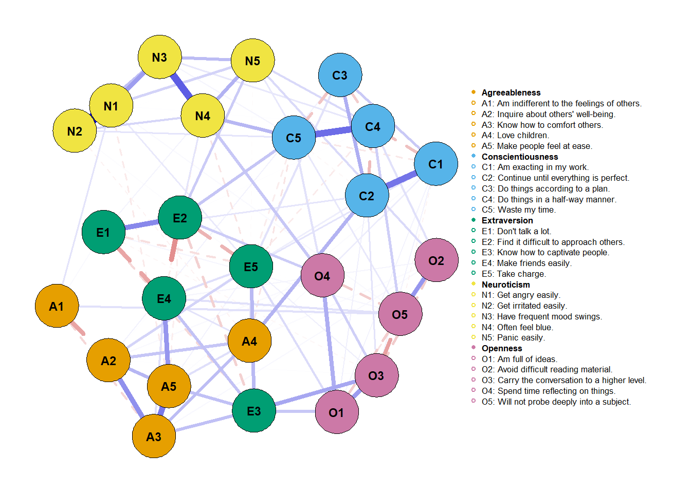
The highest edge weight is 0.53! We’ll fix both of these arguments when plotting our graphs. Now that we have that, let’s graph our networks (first Male, then the Female one):

plot(network_male, 
     layout = net_layout, #' *fixed layout*
     maximum = max_value, #' *fixed edge width*
     groups = traits,
     label.cex = 0.7, # scalar on label size
     label.color = 'black', # string on label colors
     label.prop = 0.9, # proportion of the width of the node that the label scales
     
     # Edges (pp. 33-34)
     negDashed = T, # should negative edges be dashed?
     
     # Legend (p. 35-36)
     legend.cex = 0.27, # scalar of the legend
     legend.mode = 'style2', # default is 'style1'
     nodeNames = items, # names for each node to plot in legend
     
     # Generical graphical arguments (p. 36)
     font = 2)

plot(network_female, 
     layout = net_layout,
     maximum = max_value,
     groups = traits,
     label.cex = 0.7, # scalar on label size
     label.color = 'black', # string on label colors
     label.prop = 0.9, # proportion of the width of the node that the label scales
     
     # Edges (pp. 33-34)
     negDashed = T, # should negative edges be dashed?
     
     # Legend (p. 35-36)
     legend.cex = 0.27, # scalar of the legend
     legend.mode = 'style2', # default is 'style1'
     nodeNames = items, # names for each node to plot in legend
     
     # Generical graphical arguments (p. 36)
     font = 2)

We can put both networks now side by side and make useful and more accurate comparisons. But can we be sure of these comparisons? This is a job for NetworkComparisonTest (NCT; van Borkulo et al., 2017; version 2.2.1). That’ll be job for another post. You can check that here.

Finally, you’d have to report these visualization choices. Report that maximum was fixed to the maximum absolute value considering both networks and that layout was obtained using averageLayout() with the “spring” argument. Also, as we dashed negatives and made them colorblind, that’d also be an important point to raise.

References

Burger, J., Isvoranu, A. M., Lunansky, G., Haslbeck, J. M. B., Epskamp, S., Hoekstra, R. H. A., Fried, E. I., Borsboom, D., & Blanken, T. F. (in press). Reporting standards for psychological network analyses in cross-sectional data. https://psyarxiv.com/4y9nz/

Epskamp, S., Cramer, A. O. J, Waldorp, L. J., Schmittmann, V. D., Borsboom, D. (2012). qgraph: Network visualizations of relationships in psychometric data. Journal of Statistical Software, 48(4), 1–18. https://doi.org/10.18637/jss.v048.i04

Epskamp, S., Borsboom, D., & Fried, E. I. (2017). Estimating psychological networks and their accuracy: A tutorial paper. Behavior Research Methods, 50(1), 195–212. https://doi.org/10.3758/s13428-017-0862-1

van Borkulo, C. D., Boschloo, L., Kossakowski, J. J., Tio, P., Schoevers, R. A., Borsboom, D., & Waldorp, L. J. (2017). Comparing network structures on three aspects: A permutation test. Manuscript submitted. https://doi.org/10.13140/RG.2.2.29455.38569