Estimate centrality measures by hand

Getting our network

Centrality measures are descriptive statistics of a nodes' influence and role in a network. In this tutorial we’ll learn how our main centrality measures are computed. These are:

1. Strength
2. Expected influence
3. Betweenness
4. Closeness
5. Comparing centrality values with qgraph’s centralityTable

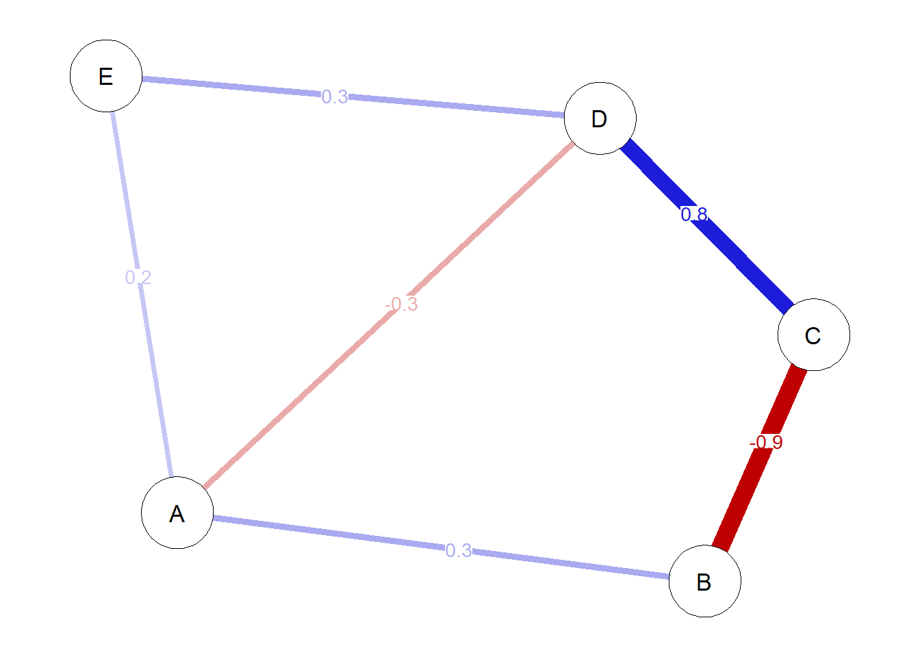
These indices will be calculated based on the following network:

if(!require("qgraph"))
    install.packages("qgraph"); library(qgraph)

# Network matrix
mat <- matrix(
  c(
       0,  0.3,    0, -0.3, 0.2,
     0.3,    0, -0.9,    0,   0,
       0, -0.9,    0,  0.8,   0,
    -0.3,    0,  0.8,    0, 0.3,
     0.2,    0,    0,  0.3,   0
  ),
  ncol = 5, nrow = 5,
  byrow = TRUE)

# Plotting network
network <- qgraph(mat,
                  layout = 'spring',
                  edge.labels = T,
                  labels = LETTERS[1:5],
                  theme = 'colorblind')

Computing strength

Strength is the easiest centrality measure to compute. Basically, it is the absolute sum of a nodes' edge weights.

Let’s do this for each node:

• Node A:
  • A–B: 0.3
  • A–D: |-0.3| = 0.3
  • A–E: 0.2
  • Strength: 0.3 + 0.3 + 0.2 = 0.8
• Node B:
  • B–A: 0.3
  • B–C: |-0.9| = 0.9
  • Strength: 0.3 + 0.9 = 1.2
• Node C:
  • C–B: |-0.9| = 0.9
  • C–D: 0.8
  • Strength: 0.9 + 0.8 = 1.7
• Node D:
  • D–A: |-0.3| = 0.3
  • D–C: 0.8
  • D–E: 0.3
  • Strength: 0.3 + 0.8 + 0.3 = 1.4
• Node E:
  • E–A: 0.2
  • E–D: 0.3
  • Strength: 0.2 + 0.3 = 0.5

Note that node C has the highest strength centrality. This means that this node has strongest connections. Also, node E has the lowest value of strength centrality, indicating a reasonably unimportant or deactivated node. These are the raw values of strength centrality. An ideal thing to do would be to standardize these indices. We can do that computing z scores for each of these measures.

This practice is the most commonly used (raw scores can be easily influenced by number of nodes, for instance). We’ll create a quick function below to help us get z scores.

get_z <- function(vector){
  mean_vector <- mean(vector)
  sd_vector <- sd(vector)
  z <- (vector - mean_vector)/sd_vector
  
  return(z)
}

strength_scores <- c(0.8, 1.2, 1.7, 1.4, 0.5)
get_z(strength_scores)

## [1] -0.6716408  0.1679102  1.2173489  0.5876857 -1.3013040

These are the z scores for strength centrality. Note that E has the lowest centrality indice and C remains as the strongest node. Here, when talking about strength, negative z scores indicate unimportant or poorly connected nodes. This interpretation is correct when we’re dealing with a fully positively connected network. However, in networks with negative edges this interpretation could be biased. We’ll see that in the next section.

Computing expected influence

Expected influence is a centrality measure suggested by Robinaugh et al. (2016) when dealing with a node’s importance in activating or deactivating other nodes in a network that has negative edges.

To calculate expected influence, we sum a node’s edge weights. This time, we don’t use absolute values. Soon we’ll understand a bit more about why.

• Node A:
  • A–B: 0.3
  • A–D: -0.3
  • A–E: 0.2
  • Expected influence: 0.3 -0.3 + 0.2 = 0.2
• Node B:
  • B–A: 0.3
  • B–C: -0.9
  • Expected influence: 0.3 - 0.9 = -0.6
• Node C:
  • C–B: -0.9
  • C–D: 0.8
  • Expected influence: -0.9 + 0.8 = 0.1
• Node D:
  • D–A: -0.3
  • D–C: 0.8
  • D–E: 0.3
  • Expected influence: -0.3 + 0.8 + 0.3 = 0.8
• Node E:
  • E–A: 0.2
  • E–D: 0.3
  • Expected influence: 0.2 + 0.3 = 0.5

Note that node D has the highest expected influence. This means that, if we wanted to activate this network, we’d aim in activating node D first. We could also note that node B has the lowest expected influence. This time, this doesn’t necessarily mean that node B is unimportant. On the contrary, node B could be activated if we wanted to deactivate our network.

Based on that, it probably is quite obvious now that, in this network, node C appears to be the most unimportant node. Why? This is because expected influence values close to 0 indicate nodes that either have very poor connections or that have ambivalent connections. In this case, node C has a strong positive connection with node D, and also a strong negative connection with node B. Say we were interested in activating node C. What would happen? Well, node C would strongly activate node D, and at the same time strongly deactivate node B. That is, its impact in the network is close to nothing since its activating one part of the network and deactivating another.

That said, z scores next to 0 represent very low impact nodes. Greater values of z scores would indicate influential nodes.

ei_scores <- c(0.2, -0.6, 0.1, 0.8, 0.5)
get_z(ei_scores)

## [1]  0.0000000 -1.5255401 -0.1906925  1.1441551  0.5720776

Computing betweenness

Betweenness indicates how many times a node is the shortest path between two other nodes. And that’s it… So, to get this value, we only need to sum how many times a specific node is in the middle (or is the shortest path) between two other nodes.

• Node A:
  • 0 times
• Node B:
  • 1 time (A–C)
• Node C:
  • 2 times (B–D, B–E)
• Node D:
  • 2 times (C–E, B–E)
• Node E:
  • 0 times

Note that B passes for two nodes before getting to E. This seems weird at first (at least to me, it sure seemed weird). This pathway is confirmed when we look at closeness centrality.

Having that, we can get z scores pretty easily.

betweenness_scores <- c(0, 1, 2, 2, 0)
get_z(betweenness_scores)

## [1] -1  0  1  1 -1

Higher scores indicate nodes that would be useful if we’re willing to “spread a message” through our network.

Computing closeness

Closeness indicates how near a node is to other nodes in the network. Say we’re interested in activating the maximum number of nodes possible. A good strategy would be to start off with the node with higher closeness centrality.

To calculate closeness centrality, we have to sum our nodes' distance. To get that, we invert the edge weight a node has with every other node and sum these values. We take this final value and again we get the inverse of that.

• Node A:
  • A–B = 0.3
  • A–C = 0.3 + |-0.8|
  • A–D = |-0.3|
  • A–E = 0.2
  • Closeness = 1/((1/0.3) + (1/0.3 + 1/0.8) + (1/0.3) + (1/0.2)) = 0.06153846
• Node B:
  • B–A = 0.3
  • B–C = |-0.9|
  • B–D = |-0.9| + 0.8
  • B–E = |-0.9| + 0.8 + 0.3
  • Closeness = 1/((1/0.3) + (1/0.9) + (1/0.9 + 1/0.8) + (1/0.9 + 1/0.8 + 1/0.3)) = 0.08000000
• Node C:
  • C–A = |-0.9| + 0.3
  • C–B = |-0.9|
  • C–D = 0.8
  • C–E = 0.8 + 0.3
  • Closeness = 1/((1/0.9 + 1/0.3) + (1/0.9) + (1/0.8) + (1/0.8 + 1/0.3)) = 0.06153846
• Node D:
  • D–A = |-0.3|
  • D–B = 0.8 + |-0.9|
  • D–C = 0.8
  • D–E = 0.3
  • Closeness = 1/((1/0.3) + (1/0.8 + 1/0.9) + (1/0.8) + (1/0.3)) = 0.0972973
• Node E:
  • E–A = 0.2
  • E–B = 0.3 + 0.8 + |-0.9|
  • E–C = 0.3 + 0.8
  • E–D = 0.3
  • Closeness = 1/((1/0.2) + (1/0.3 + 1/0.8 + 1/0.9) + (1/0.3 + 1/0.8) + (1/0.3)) = 0.05373134

The node with highest closeness value is node D, again proving to be an important node in this network. The node with lowest closeness centrality is node E - indeed the furthest node from the network. Again, we standardize these indices to get z values:

closeness_scores <- c(0.06153846, 0.08000000, 0.06153846, 0.0972973, 0.05373134)
get_z(closeness_scores)

## [1] -0.5251825  0.5193119 -0.5251825  1.4979374 -0.9668843

Comparing centrality values

Did we do it right? Instead of computing all these values, we generally just ask for a quick summary using centralityTable or centralityPlot. To get standardized values (z scores), the argument standardized must be TRUE (this is the default).

centralityTable(network)

##      graph type node           measure       value
## 1  graph 1   NA    A       Betweenness -1.00000000
## 2  graph 1   NA    B       Betweenness  0.00000000
## 3  graph 1   NA    C       Betweenness  1.00000000
## 4  graph 1   NA    D       Betweenness  1.00000000
## 5  graph 1   NA    E       Betweenness -1.00000000
## 6  graph 1   NA    A         Closeness -0.80202257
## 7  graph 1   NA    B         Closeness  0.21659584
## 8  graph 1   NA    C         Closeness  0.64723127
## 9  graph 1   NA    D         Closeness  1.17097705
## 10 graph 1   NA    E         Closeness -1.23278160
## 11 graph 1   NA    A          Strength -0.67164077
## 12 graph 1   NA    B          Strength  0.16791019
## 13 graph 1   NA    C          Strength  1.21734889
## 14 graph 1   NA    D          Strength  0.58768567
## 15 graph 1   NA    E          Strength -1.30130399
## 16 graph 1   NA    A ExpectedInfluence  0.07389689
## 17 graph 1   NA    B ExpectedInfluence -1.40404097
## 18 graph 1   NA    C ExpectedInfluence -0.48032981
## 19 graph 1   NA    D ExpectedInfluence  1.18235029
## 20 graph 1   NA    E ExpectedInfluence  0.62812359

Instead of reporting each centrality indice, we can ask for a plot. Let’s sort the nodes from highest to lowest expected influence values.

centralityPlot(network, include = "all", orderBy = "ExpectedInfluence")

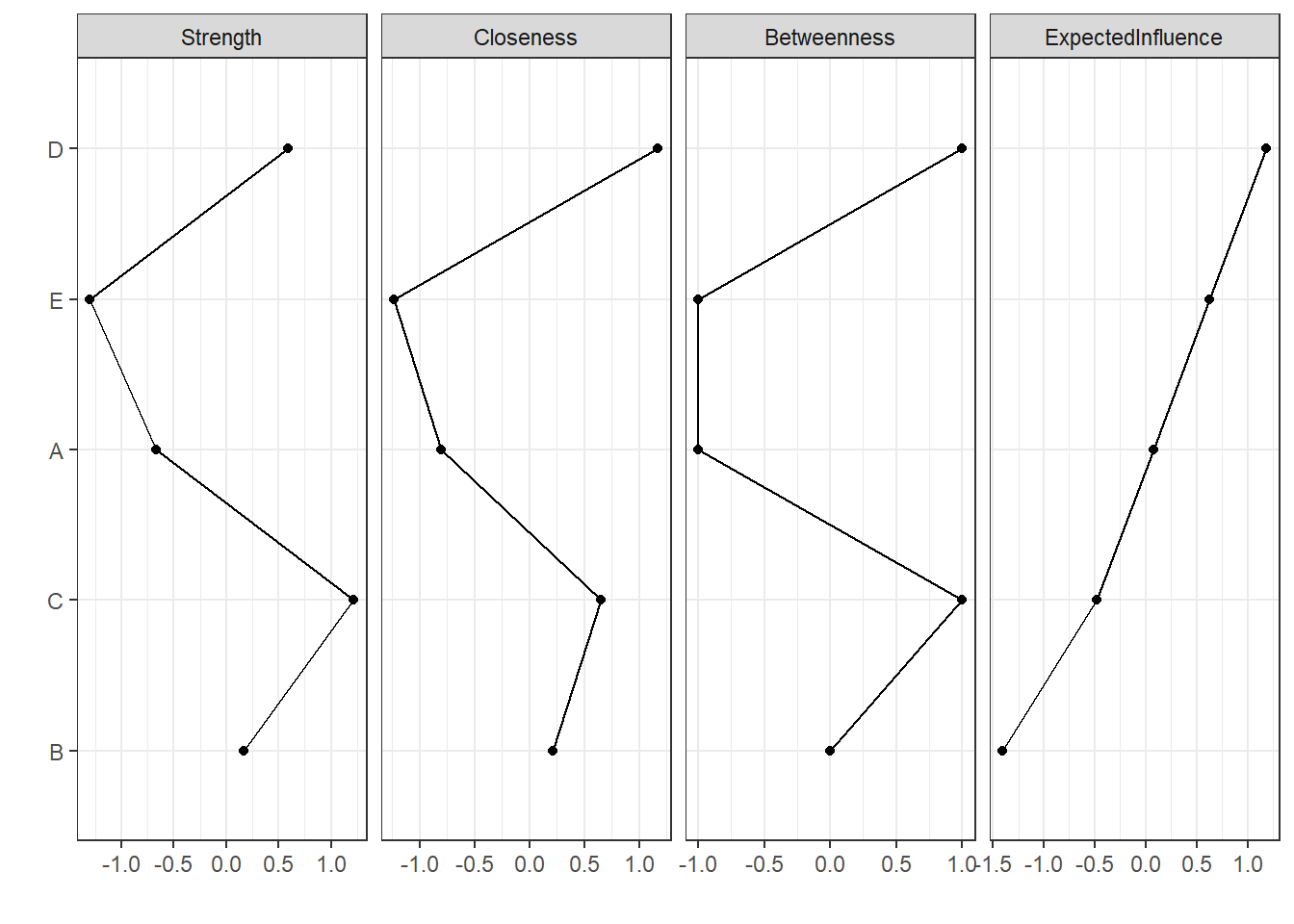
From this plot, it’s become very apparent that node D seems to be very influential in this network.

References

Costantini, G., Epskamp, S., Borsboom, D., Perugini, M., Mõttus, R., Waldorp, L. J., & Cramer, A. O. J. (2015). State of the aRt personality research: A tutorial on network analysis of personality data in R. Journal of Research in Personality, 54, 13–29. https://doi.org/10.1016/j.jrp.2014.07.003

Epskamp, S., Cramer, A. O. J, Waldorp, L. J., Schmittmann, V. D., Borsboom, D. (2012). qgraph: Network visualizations of relationships in psychometric data. Journal of Statistical Software, 48(4), 1–18. https://doi.org/10.18637/jss.v048.i04

Epskamp, S., Borsboom, D., & Fried, E. I. (2017). Estimating psychological networks and their accuracy: A tutorial paper. Behavior Research Methods, 50(1), 195–212. https://doi.org/10.3758/s13428-017-0862-1

Robinaugh, D. J., Millner, A. J., & McNally, R. J. (2016). Identifying highly influential nodes in the complicated grief network. Journal of Abnormal Psychology, 125(6), 747–757. http://doi.org/10.1037/abn0000181.